###################============== Loading Packages =============== ==== #################
library(plyr) # Rmisc association package, if you need to load dplyr package at the same time, you must first load the plyr package.
library(dplyr) # filter()
library(ggplot2) # ggplot()
library(DT) # datatable() Create an interactive data table
library(caret) # createDataPartition() stratified sampling function
library(rpart) # rpart()
library(e1071) # naiveBayes()
library(pROC) # roc()
library(Rmisc) # multiplot() Split drawing area
################### ============= Import data ================ == #################
hr <- read.csv("D:/R/天善智能/书豪å大案例/Employee turnover prediction \\HR_comma_sep.csv")
str(hr) # View the basic data structure of the data
Descriptive analysis
################### ============= Descriptive Analysis ================ === ###############
str(hr) # View the basic data structure of the data
summary(hr) # Calculate the main descriptive statistics of the data
# subsequent individual models need the target variable to be factor type, we convert it to factor type
hr$left <- factor(hr$left, levels = c('0', '1'))
## Exploring the relationship between employee satisfaction, performance evaluation, and average monthly working hours and resignation
# Draw a box plot of satisfaction with the company and whether or not to leave
box_sat <- ggplot(hr, aes(x = left, y = satisfaction_level, fill = left)) +
geom_boxplot() +
theme_bw() + # a ggplot theme
labs(x = 'left', y = 'satisfaction_level') # Set the horizontal and vertical coordinates
box_sat
Box line chart of employee satisfaction with the company and whether or not to leave
Retired employees are less satisfied with the company, mostly concentrated around 0.4;
# Draw a performance assessment and a box line diagram of whether to leave
box_eva <- ggplot(hr, aes(x = left, y = last_evaluation, fill = left)) +
geom_boxplot() +
theme_bw() +
labs(x = 'left', y = 'last_evaluation')
box_eva
Performance appraisal and box line diagram of resignation
The performance evaluation of the departing employees is higher, and the concentration is above 0.8;
# Draw a box plot of the average monthly working hours and whether or not to leave
box_mon <- ggplot(hr, aes(x = left, y = average_montly_hours, fill = left)) +
geom_boxplot() +
theme_bw() +
labs(x = 'left', y = 'average_montly_hours')
box_mon
The average monthly working hours of retired employees is higher, more than half of the average (200 hours)
# Draw a box plot of the employee's working years in the company and whether or not to leave
box_time <- ggplot(hr, aes(x = left, y = time_spend_company, fill = left)) +
geom_boxplot() +
theme_bw() +
labs(x = 'left', y = 'time_spend_company')
box_time
The working years of the departing employees are around 4 years.
# Combine these graphics in a drawing area, cols = 2 means that the layout is a row and two columns
multiplot(box_sat, box_eva, box_mon, box_time, cols = 2)
## Explore the number of participating projects, whether there is promotion in five years, and the relationship between salary and turnover
# Need to convert this variable into a factor type when drawing a bar chart of participating items
hr$number_project <- factor(hr$number_project,
levels = c('2', '3', '4', '5', '6', '7'))
# Draw the number of participating projects and whether or not to leave the percentage of the stacked bar chart
bar_pro <- ggplot(hr, aes(x = number_project, fill = left)) +
geom_bar(position = 'fill') + # position = 'fill' is to draw a percentage stacked bar chart
theme_bw() +
labs(x = 'left', y = 'number_project')
bar_pro
Employees participating in the number of projects and the percentage of whether they left the stacked bar chart
The more employees attending the project, the greater the turnover rate of employees (samples with 2 items removed)
# Draw a percentage bar chart of whether to promote and resign within 5 years
bar_5years <- ggplot(hr, aes(x = as.factor(promotion_last_5years), fill = left)) +
geom_bar(position = 'fill') +
theme_bw() +
labs(x = 'left', y = 'promotion_last_5years')
bar_5years
Percentage bar chart of whether to promote and resign within 5 years
The turnover rate of employees who have not been promoted within five years is relatively large.
# Plot the salary and the percentage of the resignation stacked bar chart
bar_salary <- ggplot(hr, aes(x = salary, fill = left)) +
geom_bar(position = 'fill') +
theme_bw() +
labs(x = 'left', y = 'salary')
bar_salary
Payroll and percentage of whether or not to leave a stacked bar chart
The higher the salary, the lower the turnover rate
# Combine these graphics in a drawing area, cols = 3 means that the layout is a row and three columns
multiplot(bar_pro, bar_5years, bar_salary, cols = 3)
Modeling prediction regression tree
############## =============== Extracting Excellent Employees =========== ####### ############
# filter() is used to filter the eligible samples
hr_model <- filter(hr, last_evaluation >= 0.70 | time_spend_company >= 4
| number_project > 5)
############### ============ Custom cross-validation method ========== ######## ##########
# Set 5-fold cross-validation method = 'cv' is to set the cross-validation method, number = 5 means 5-fold cross-validation
train_control <- trainControl(method = 'cv', number = 5)
################ =========== Divided into samples ============== ####### ###################
set.seed(1234) # Set random seeds in order to make the results consistent for each sample
# 7:3 stratified sampling based on the dependent variable of the data, returning the row index vector p = 0.7 means sampling according to 7:3,
#list=FI will not return the list, return vector
index <- createDataPartition(hr_model$left, p = 0.7, list = F)
traindata <- hr_model[index, ] # extracts the data of the index corresponding to the index in the data as a training set
testdata <- hr_model[-index, ] # rest as a test set
#####################================================================================================= ####################
# Using the train function in the caret package to establish a decision tree model using the 5-fold crossover method for the training set
# left ~. Means modeling from dependent variables and all independent variables; trControl is the control used to model
# methon is to set which algorithm to use
rpartmodel <- train(left ~ ., data = traindata,
trControl = train_control, method = 'rpart')
# Use the rpartmodel model to predict the test set, ([-7] means to eliminate the dependent variable of the test set)
pred_rpart <- predict(rpartmodel, testdata[-7])
#Create confusion matrix, positive='1' set our positive example to "1"
con_rpart <- table(pred_rpart, testdata$left)
con_rpart
Modeling prediction of naive Bayes
###################============ Naives Bayes =============== ## ###############
nbmodel <- train(left ~ ., data = traindata,
trControl = train_control, method = 'nb')
pred_nb <- predict(nbmodel, testdata[-7])
con_nb <- table(pred_nb, testdata$left)
con_nb
Model evaluation + application
##################====================================================================== ====== #################
# When using the roc function, the predicted value must be numeric
pred_rpart <- as.numeric(as.character(pred_rpart))
pred_nb <- as.numeric(as.character(pred_nb))
roc_rpart <- roc(testdata$left, pred_rpart) # Get the information used in subsequent drawing
#False positive rate: (1-Specificity[)
Specificity <- roc_rpart$specificities # lays the foundation for the subsequent horizontal and vertical axis, true counterexample rate
Sensitivity <- roc_rpart$sensitivities # recall rate: sensitivities, also true case rate
#draw ROC curve
#we only need the horizontal and vertical coordinates NULL is to declare that we are not using any data
p_rpart <- ggplot(data = NULL, aes(x = 1- Specificity, y = Sensitivity)) +
geom_line(colour = 'red') + # Draw ROC curve
geom_abline() + # draw diagonal
annotate('text', x = 0.4, y = 0.5, label = paste('AUC=', #text is a text comment on the declaration layer
#'3' is a parameter inside the round function, retaining three decimal places
round(roc_rpart$auc, 3))) + theme_bw() + # Add AUC value in the figure (0.4, 0.5)
labs(x = '1 - Specificity', y = 'Sensitivities') # Set the horizontal and vertical axis labels
p_rpart
Returning tree ROC curve
roc_nb <- roc(testdata$left, pred_nb)
Specificity <- roc_nb$specificities
Sensitivity <- roc_nb$sensitivities
p_nb <- ggplot(data = NULL, aes(x = 1- Specificity, y = Sensitivity)) +
geom_line(colour = 'red') + geom_abline() +
annotate('text', x = 0.4, y = 0.5, label = paste('AUC=',
round(roc_nb$auc, 3))) + theme_bw() +
labs(x = '1 - Specificity', y = 'Sensitivities')
p_nb
Naive Bayes ROC Curve
AUC value of the regression tree (0.93) > AUC value of naive Bayes (0.839)
Finally, we chose the regression tree model as our actual prediction model.
###############################==================================================================== ==####################
# Use the regression tree model to predict the probability of classification, type='prob' set the prediction result as the probability of leaving the job and the probability of not leaving the job.
pred_end <- predict(rpartmodel, testdata[-7], type = 'prob')
# Combined forecast results and predicted probability results
data_end <- cbind(round(pred_end, 3), pred_rpart)
# Rename the forecast results table
names(data_end) <- c('pred.0', 'pred.1', 'pred')
# Generate an interactive data table
datatable(data_end)
Finally we will generate a forecast result table
Antenk DIN41612 Connectors are a versatile two piece PCB connector set with feaures useful for many applications including connections for plug-in card and back-panel wiring, PCB to PCB attachment and peripheral connections for external interfaces. Features include a multitude of body sizes and styles with options that include selective contact loading, make and break contacts, contact lead length choices and contact plating variations each in .100" [2.54mm] or .200" [5.08mm] centerline spacing.
The DIN 41612 standard covers a series of two-piece backplane connectors widely used in rack-based telecommunication, computing, process control, medical, industrial automation, test and measurement and military/aerospace systems where long-term reliability is required. They consist of one to three rows of contacts in combinations of 16, 32, 48, 64, or 96 contacts on a 0.1-inch (2.54 mm) grid pitch. The 3 rows are labelled a, b and c and connectors up to 64 way if using a 96 way body can use either rows a+b or a+c. DIN 41612 Signal connectors can be rated to 1.5 amps per signal pin, at 500 volts, although these figures may be de-rated according to safety requirements or environmental conditions. Several hybrid power and coaxial configurations are available that can handle up to 5.6A or even 15A. This wealth of variations explains the very wide range of applications that they`re put to. For over 30 years these DIN 41612 `Euro Card` connectors to IEC 60603-2 have offered a highly reliable system for board interconnects. Precision contact density, low mating forces, a two piece protective design and many contact termination styles offer unlimited design opportunities. Termination methods include – straight PC, solder eyelet, wire wrap, crimp and [press fit" terminals. Insertion and removal force are controlled, and three durability grades are available. Standardisation of the connectors is a prerequisite for open systems, where users expect components from different suppliers to operate together; ept and Conec DIN 41612 are therefore fully intermateable with all other similarly compliant products from other manufacturers like Harting, Erni, Hirose and TE Connectivity, etc.
The most common connector in the DIN product line is type C, which is widely used in VMEbus systems, the DIN 41612 standard has been upgraded to meet international standards IEC 60603-2 and EN 60603-2. In the past, ept used a comb supported press-fit tool for their type C and B press-fit female connectors. To be more competitive, ept has changed to flat-rock technology (just a flat piece of steel pushed on the top of the connector) as used by many other manufacturers.
DIN 41612 Connectors are widely used in rack-based electrical systems. The standard performance of these connectors is a 2 A per pin current carrying capacity and 500 V working voltage. Both figures may be variable due to safety and environmental conditions.
Types
Number of contacts varies
Many variations of housing material, including different types of metal and plastic
Both angled and straight versions
Male and female
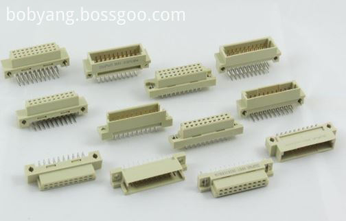
C,R,B,Q Type DIN41612 Connectors

Half C, R, B & Q Type DIN41612 Connectors

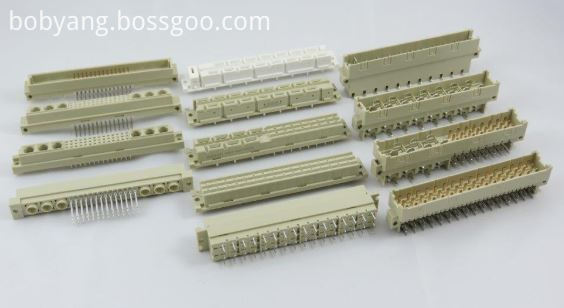
1/3 C,R, B & Q Type DIN41612 Connectors

H, F, H+F & M type DIN41612 Connectors

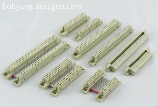
IDC Type DIN41612 Connectors

Female Cable Connector

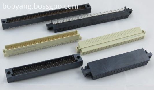
High Pin Count DIN41612 Connectors

Shroud DIN41612 Connectors

Features and Benefits of Din41612 Connector:
• Indirect mating (male/female)
• Automated production processes
• Continuous quality assurance
• 3-160 contacts
• Complete interconnection system
• Numerous interface connectors
• A wide variety of hoods
• Many termination technologies provide for the lowest installed cost
• Contacts selectively gold-plated
• Tinned terminations for increased solderability
Uses
The primary use of DIN 41612 connectors are PCB Connectors and motherboards, the main acceptance would be their board to board reliable connections.
Applications of Din41612 Connector:
Applications
• Data centers
• Storage
• Servers
• Base stations
• Telecommunications equipment
• Backplane and motherboard assemblies
• Switching systems
• Modular rack systems
• Power automation
• Distributed control systems in
industrial control
• Programmable logic controllers (PLC)
• Robotics
• Test and lab equipment
• Energy distribution
• Monitoring equipment
This is not a definitive list of applications for this product. It represents some of the more common uses.
Din41612 Connectors,Din 41612,Eurocard Connector Din41612,Male Din41612 Connector
ShenZhen Antenk Electronics Co,Ltd , https://www.antenk.com